Introduction & Motivation
In my own experience with systematic trading education, I repeatedly encountered parameter tuning presented as a self-evident and almost unquestioned step in strategy development. While the technical execution of optimization was often demonstrated in detail (grid search), considerably less attention was paid to whether this tuning truly works in practice — or the configurations are stable, resilient, and predictive out-of-sample.. This raises several fundamental questions that form the core motivation of this project.
Problem Statement & Research Questions
Before diving into the analysis, it is important to clarify what kind of research questions this project addresses and which it does not. In particular, I will not investigate whether optimized MACD parameters provide predictive value for out-of-sample (OOS) trading performance or whether they can be directly used for live trading. Instead, the focus is on understanding the pattern, persistence, and evolution of the best-performing configurations over time. Questions outside this scope will be discussed briefly in the conclusion to guide further research for those who are interested in this topic and want to build their own trading strategies based on parameter optimization.
Hypothesis & Research Questions
To sum up, the main hypothesis and research questions are as follows:
-
➣
Hypothesis 1
Historical price data may contain exploitable structure and patterns that can be captured by systematic trading rules.
Assuming Hypothesis 1 holds at least in some contexts, the analysis focuses on the following questions:
-
➣
Research Question 1
Does a locally high-performing region exist in the configuration space? -
➣
Research Question 2
How does this region change, drift or deform over time?
Assumptions & Framing
-
➣
Methodological Framing
Parameter optimization is treated as a model selection problem conditional on a specific strategy, asset, timeframe, and evaluation metric. The selected configurations are not interpreted as profit guarantees but as historically high-performing setups whose patterns, consistency, and potential deterioration are studied using fixed-size sliding windows. -
➣
Assumption on Market Dynamics
This framework accounts for non-stationary market conditions. The fixed sliding windows implicitly test whether locally stable regimes exist, how long they persist, and how parameter structures change or drift as these regimes evolve.
Under these assumptions, the core objective of this project is not to identify a single “best” parameter set, but to explore the behavior, stability, and evolution of optimized parameters across time and data slices.
Methodology
This study is conducted within a fully reproducible, programmatic research environment designed to evaluate parameter behavior under controlled conditions. All simulations are executed using a consistent execution model, data source, and evaluation pipeline in order to isolate the effects of parameter choice and temporal structure.
Data Source & Asset Selection
Historical market data is sourced from Yahoo Finance and consists of daily OHLCV bars for the BTC-USD trading pair spanning the period from 2021-01-02 to 2025-12-31 (1825 days).
BTC-USD is selected as the sole asset for this analysis for several reasons:
- ➣ Continuous trading: The market operates 24/7, eliminating artificial return discontinuities caused by market closures, making it particularly suitable for time-series analysis and rolling-window experimentation;
- ➣ High liquidity and global participation: BTC exhibits deep liquidity and broad market involvement across regimes;
- ➣ Distinct regime shifts: The dataset includes multiple bull, bear, and sideways market phases, providing a rich environment to study parameter stability and degradation.
The choice of a single, well-understood asset is intentional: the objective of this research is not cross-asset generalization, but rather a controlled examination of parameter behavior under varying temporal contexts. However, I developed the codebase with flexibility in mind, allowing for easy extension to additional assets, timeframe or even different trading strategies.
Backtesting Framework
All simulations are performed using the VectorBT backtesting Python library, which enables fast, vectorized evaluation of large parameter grids under a consistent execution model. The framework is used in a signal-based configuration, where entry and exit conditions are derived directly from indicator state transitions.
To ensure comparability across simulations, transaction costs, slippage assumptions, and position sizing rules are held constant throughout the experiment.
Strategy Definition
The strategy is not designed to maximize returns but serves as a controlled and interpretable vehicle for exploring configuration behavior over time. As such, the strategy is intentionally simple and well-known.
Indicator
The strategy is based on the Moving Average Convergence Divergence (MACD) indicator, specifically focusing on the MACD histogram, defined as the difference between the MACD line and its associated signal line.
The MACD is parameterized by three integer values:
- ➣ Fast period: short-term Exponential Moving Average (EMA) length — notated as \( EMA_{fast} \)
- ➣ Slow period: long-term EMA length — notated as \( EMA_{slow} \)
- ➣ Signal period smoothing length applied to the MACD line — notated as \( EMA_{signal} \)
Trading Logic
The strategy utilizes the momentum effect in a way that operates in a long-only configuration and generates trading signals based on sign changes in the MACD histogram:
- ➣ Entry: A long position is opened when the MACD histogram transitions from negative to positive i.e. when the MACD line crosses above its signal line.
- ➣ Exit: The position is closed when the MACD histogram transitions from positive to negative i.e. when the MACD line crosses below its signal line.
No leverage, short selling, or additional filters are applied.
Parameter Space & Hierarchical Optimization Design
The experimental design of this study operates over two distinct but interacting parameter spaces. The first corresponds to the intrinsic MACD indicator parameters, which define the mathematical behavior of the signal itself. The second represents a higher-level temporal configuration space, governing how the historical price series is segmented into rolling and overlapping evaluation windows. Together, these form a hierarchical grid designed to assess not only performance but also temporal robustness and configuration reliability.
MACD Parameter Grid
As noted earlier, the MACD configuration space explored encompasses a wide range of integer values for the three MACD parameters. Note that I applied 2 constraints which filters out invalid configurations to ensure logical consistency in the parameter combinations:
- ➣ The fast period must be less than the slow period. This is a fundamental requirement for the MACD calculation, as the fast EMA is intended to capture short-term momentum relative to the longer-term trend represented by the slow EMA, otherwise they wouldn't be called "fast" and "slow".
- ➣ The signal period must be less than the slow period. This is not strictly required for MACD calculation, but using a longer signal period would oversmooth the already smoothed MACD line, reducing the histogram's responsiveness to momentum shifts.
Temporal Window Configuration Space (Meta-Parameters)
Beyond indicator-level parameters, this research introduces a second, higher-order configuration space governing the temporal segmentation of historical data. Instead of evaluating MACD parameters over a single fixed backtest interval, the full study period from 2021-01-02 to 2025-12-31 is decomposed into multiple overlapping time windows.
Concretely, fixed-length windows of 730 days are used and shifted forward in increments of 73 days (approximately two months). This results in 15 distinct starting points across the full period, meaning that the entire MACD parameter grid is evaluated independently within each temporal slice.
These window configurations function as meta-parameters: they define the temporal context and implicit market regime under which each parameter set is evaluated. By comparing the structure of optimal regions across windows, the analysis aims to distinguish between locally stable parameter structures and configurations that only perform well within a specific historical phase.
It is important to emphasize that fixed-length windows are unlikely to represent the theoretically optimal way of segmenting market history. Parameter optima are expected to shift primarily during regime transitions or when the underlying market characteristics materially change. A regime-based segmentation might therefore be more appropriate in principle. However, regime identification itself constitutes a separate and non-trivial research problem. In particular, determining regime boundaries in real time — rather than retrospectively — is substantially more difficult, since ex-post analysis makes structural breaks appear clearer than they are in practice. It's the typical case of "easy to be smart after the fact".
The chosen 730-day window length is intentionally longer than a typical macro trend cycle, implying that individual windows likely contain multiple overlapping regimes. This design choice is accepted as a simplifying assumption for the current study, prioritizing structural comparability across time slices over precise regime isolation. Furthermore, I specificly selected quite short shifts (73 days) to ensure that the windows are highly overlapping, which allows for a more granular analysis of how parameter structures evolve as the market transitions through different phases.
Additionally, each window includes a padding period prior to its formal start date in order to initialize indicator values properly. Since MACD requires a warm-up phase equal to the sum of its slow and signal periods, this padding ensures that early-window signals are not distorted by incomplete historical data.
Configuration Summary
Configuration Summary Table
All configurations are summarized in the table below like data, strategy, simulation meta-parameters, trade execution assumptions etc.
| Parameter | Value | Description |
|---|---|---|
| Asset | BTC-USD | Asset being traded in the backtest simulations. |
| Data Source | Yahoo Finance | Provider of historical OHLCV price data. |
| Timeframe | Daily bars | Resolution of the price data used for backtesting. |
| Full Study Period | 2021-01-02 to 2025-12-31 | Overall date range for all backtest simulations. |
| MACD Parameters |
\( EMA_{fast} \): 2-50 (step 2) \( EMA_{slow} \): 20-200 (step 2) \( EMA_{signal} \): 2-100 (step 2) |
Ranges and step sizes for MACD indicator parameters. |
| Initial Capital | $1,000 | Starting equity for each backtest simulation. |
| Transaction Costs | 0.1% per trade | Fixed cost applied to each buy and sell transaction. |
| Slippage | 0.1% per trade | Assumed market impact cost for each transaction. |
| Position Sizing | 100% of equity | Full capital is allocated to each trade. |
| Trade Direction | Long-only | Strategy only takes long positions; no short selling. |
| Temporal Windows |
length: 730 days shift: 73 days |
Rolling window length and its respective shifts used for backtesting. |
Performance Metrics & Structural Selection Criteria
Before delving into the analysis part, it is important to clarify what is considered as "optimal". The choice of objective function directly influences the parameter selection process and the subsequent interpretation of results. In order to select a "good" objective function, one has to analyze the properties and statistical behaviour of their concrete configuration. In this study, it's not the main focus of the project therefore I will rely on intuition and visual confirmation when selecting the objective function, but I will also briefly discuss what one should keep in my mind if they want to develop their own strategy for actual trading.
Defining Optimality
In the context of this research, “optimality” does not simply mean the highest numerical value of a performance metric. Instead, t refers to structural properties of the configuration space under a given metric. Since the primary goal of this project is to analyze the existence and stability of locally optimal regions in the MACD parameter space, the chosen objective function must support meaningful structural interpretation.
Concretely, an objective function is considered suitable if it satisfies the following practical criteria:
- ➣ Comparability: All parameter combinations should yield finite and comparable values. Metrics that can become undefined or explode to extreme values (e.g., due to division by zero or very few trades) distort the structure of the parameter space.
- ➣ Structural smoothness: The metric surface over the parameter grid should not be dominated by a small number of isolated outliers. Instead, high-performing regions should form relatively smooth and coherent clusters.
- ➣ Separation quality: The metric should produce clearly distinguishable regions of high and low performance. If multiple disconnected regions appear equally strong without clear structure, it becomes difficult to identify meaningful local optima.
- ➣ Cross-metric consistency: High-performing areas under the selected metric should not directly contradict other fundamental risk or return measures. While perfect correlation is not expected, extreme disagreement (for example, excellent score combined with structurally poor drawdown behavior) would indicate instability in the definition of optimality.
Under this definition, optimality is therefore interpreted as the presence of a concentrated, internally coherent, and reasonably consistent high-performance region within the parameter space — rather than the existence of a single isolated peak value.
Importantly, this definition is operational and project-specific. It is not derived from formal statistical testing, nor does it claim theoretical superiority. The objective function is evaluated primarily through structural inspection of the parameter grid across rolling windows, since the central research question concerns stability and spatial organization, not the universal validity of a particular performance metric.
Considered metrics & My Choice
Sharpe Ratio
The Sharpe Ratio measures excess return compared to a risk free investment per unit of total volatility:
\[ \text{Sharpe} = \frac{\mathbb{E}[\mathbf{R} - \mathbf{R}_f]}{\sigma(\mathbf{R})} \]
While theoretically appealing as a risk-adjusted return measure and it's one of the most wildly chosen leading metric, in this parameter grid it frequently produced noisy heatmap in the MACD spaces and a single optimal region was not clearly distinguishable.
Sortino Ratio
The Sortino Ratio refines Sharpe by penalizing only downside volatility:
\[ \text{Sortino} = \frac{\mathbb{E}[\mathbf{R} - \mathbf{R}_f]}{\sigma_{\text{downside}}(\mathbf{R})} \]
Although conceptually more aligned with asymmetric risk perception mainly if the selected asset has strong upside skewness, it exhibited similar instability issues.
Max Drawdown
Maximum Drawdown measures the largest peak-to-trough equity decline.
This metric presents several limitations as a primary objective function. It captures only the single worst drawdown event, making it highly sensitive to outliers and not necessarily representative of overall risk characteristics. It may even favor parameter sets that barely trade or remain inactive for extended periods, simply because they avoid large equity swings. Furthermore, the locations of its “optimal” regions often showed weak alignment with other performance metrics, suggesting structural instability within the parameter space. Finally, maximum drawdown is entirely disconnected from return generation — which becomes problematic if the ultimate goal is to make money. 🙂
Calmar Ratio
The Calmar Ratio relates return to maximum drawdown:
\[ \text{Calmar} = \frac{\text{Annualized Return}}{\text{Max Drawdown}} \]
Since the denominator is maximum drawdown, the metric inherently inherits its structural weaknesses. Because maximum drawdown is path-dependent and driven by a single extreme event, the Calmar Ratio can become highly sensitive to isolated equity shocks. In the parameter grid this frequently resulted in noisy landscapes or sharply isolated optimal regions, rather than smooth and coherent structures. Configurations with broadly similar return profiles sometimes appeared materially different solely due to one extreme drawdown event, reducing stability and interpretability across windows.
Omega Ratio
The Omega Ratio evaluates the ratio of gains to losses relative to a chosen threshold:
\[ \text{Omega} = \int_{\tau}^{\infty} (1 - F(x)) \, dx \bigg/ \int_{-\infty}^{\tau} F(x) \, dx \]
Although theoretically appealing due to incorporating the entire return distribution, in practice it did not provide sufficiently strong separation across the parameter space. The resulting surfaces often lacked a clearly dominant region and instead produced multiple scattered “islands” of locally high values. Similar to Sharpe and Sortino, the scale was not stretched in a way that would highlight one structurally superior configuration. This reduced interpretability and made structural comparisons across windows less conclusive.
Profit Factor
Profit Factor is defined as the ratio of gross profits to gross losses:
\[ \text{Profit Factor} = \frac{\text{Gross Profit}}{\text{Gross Loss}} \]
Although intuitive and trade-based, it tended to explode for parameter sets with very few losing trades for 0 losing trades it yields infinity. This created extreme outliers and reduced comparability across the grid.
Total Return
Total Return measures cumulative percentage growth over the window.
Despite being simple and interpretable, it ignores trade distribution characteristics and doesn't account for risk at all. In the parameter grid, it showed noisy landscapes with multiple scattered peaks, making it difficult to identify a single structurally superior region. Additionally, it sometimes produced high values for parameter sets that had poor drawdown profiles, indicating a lack of cross-metric consistency.
Expectancy
Finally, the expectancy measures the average expected profit per trade:
\[ \text{Expectancy} = (\text{Win Rate} \times \text{Avg Win}) - (\text{Loss Rate} \times \text{Avg Loss}) \]
In contrast to the other metrics, expectancy produced relatively smooth and coherent high-performance regions within the parameter grid. It remained finite for all configurations, reduced extreme outlier effects, and demonstrated reasonable alignment with return-based metrics while avoiding strong contradiction with drawdown behaviour.
Most importantly, it generated well-defined clusters of locally optimal parameter combinations rather than isolated numerical spikes or multiple scattered peaks. For the purposes of structural and stability analysis, this made expectancy the most suitable objective function in this study.
Visual Comparison
In the interest of transparency and completeness, I am including the full set of metric heatmaps for the last window configuration as a visual reference. This allows readers to see the structural differences across metrics and understand why expectancy was selected as the primary objective function for the subsequent analysis.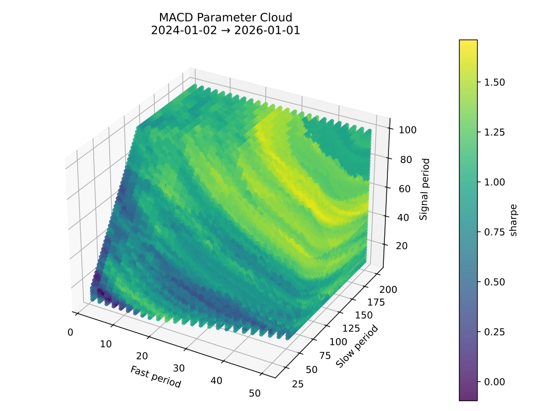
Structural Analysis of the Parameter Space
In this section, I will present my approach to analyzing the structure of the parameter space and the stability of optimal regions across time. The analysis is based on visual inspections of the heatmaps, where I created an interatice 3D plot to explore the parameter space in more detail and I also investigated how the MACD parameters behave in pairs eliminating the third one. I will also present some quantitative measures of stability and structural consistency of top-N configurations across windows such as how the centroids shift or how they expand or contract across time. As I previously mentioned, I will present these analysis through the
Heatmap Analysis & 3D Visualization
At the end of the previous chapter, I have already included the heatmaps of different metrics for the same window which highlighted there are high-performing regions even with a naive fixed window approach. They are sometimes not perfectly smooth but definitely some structure appears. To further investigate this structure, firstly, I want to show how the parameters behave in pairs, eliminating the third one. This means an orthogonal projection of the 3D parameter space into 2D planes along the axes of the frame.
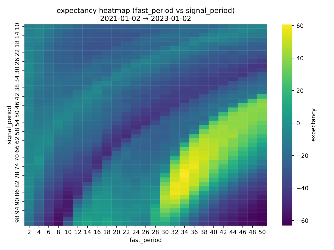
To eliminate the third parameter, the third parameter was averaged out, producing projections onto the principal planes: Fast-Signal (slow averaged), Fast-Slow (signal averaged), and Slow-Signal (fast averaged). These projections reveal a clear structural distinction: the Fast-Signal and Slow-Signal planes display an oval-shaped optimal region, indicating some tolerance and correlation between the parameters, whereas the Fast-Slow plane forms a compact, point-like region. This suggests that the signal period provides flexibility in shaping the optimum, while the relative fast–slow relationship is tightly constrained, highlighting the critical role of the momentum differential in the strategy's performance.
Finally, this section includes an interactive 3D plot of the parameter space, enabling a deeper exploration of the structure and a comparison of how different metrics behave across it. This tool is particularly useful for visually confirming the presence of optimal regions and understanding the interactions between parameters in terms of performance. Users can even rotate the plot to find the best projection angle, clearly separating the optimal region from the surrounding parameter space.
Centroid Analysis
Before diving into the results, it is important to clarify the assumptions behind centroid analysis. This approach implicitly assumes that the top-N parameter sets form a roughly ellipsoidal or convex cluster, which is not always the case — especially when the N parameter is set to a high value. There are two main reasons for this: firstly, a high N can cause the optimal region to break up into isolated islands; secondly, in some 2D projections, the optimal region forms an oval-like area, which can suggest a non-convex shape. Nonetheless, computing the centroid remains a simple and insightful way to track how the average of the best-performing parameters evolves over time, providing a useful overview of trends and shifts in the parameter landscape.
In my analysis, the centroid is computed along each individual parameter dimension over time, illustrating how fast, slow, and signal configurations shift independently. Additionally, a normalized centroid drift is calculated, aggregating across all dimensions to capture overall shifts in the top-N region without focusing on single parameters.
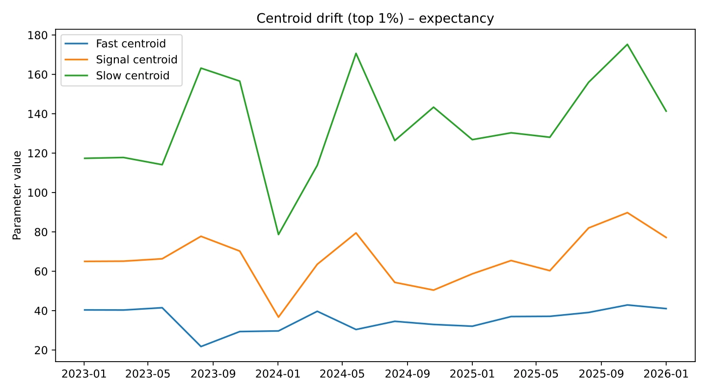
The key insight from the plots above is that the centroid of the top-N parameters shifts over time, reflecting significant changes in the optimal parameter sets as important price movements enter or exit the examined window. The individual parameter centroids exhibit a mean-reverting behaviour, indicating that the optimal region does not drift randomly but oscillates around a characteristic area in parameter space. During windows dominated by bearish or ranging periods, centroids tend to shift toward lower parameter values, whereas during strong bullish periods, they move toward higher values. This pattern suggests that the high-performing cluster is not fixed but adapts to underlying market conditions, which is consistent with the concept of regime-dependent parameter stability.
Stability Metrics
The stability of the top-N parameter sets was assessed using two complementary metrics.
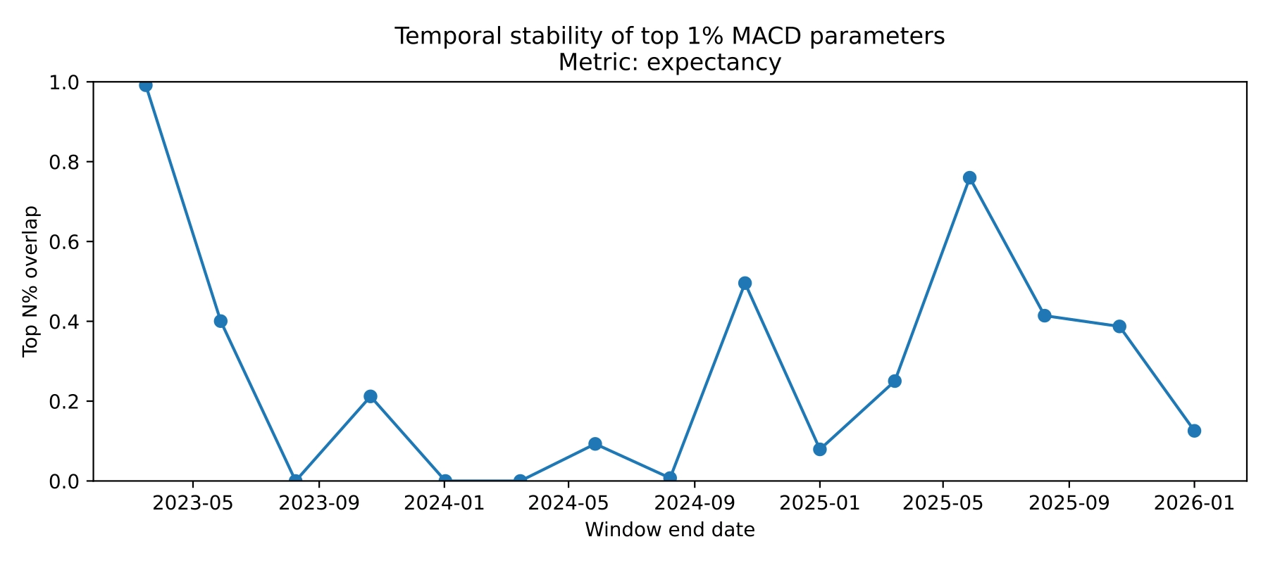
Firstly, the temporal overlap of the top-N parameters between consecutive windows was measured. This metric has the advantage of not relying on any assumptions about the shape of the optimal region, as it directly evaluates the overlap of discrete points in the parameter space. For example, for a chosen top-N region with N=1%, the plot shows how many of the top 1% parameters remained in the top 1% region of the next window. A high overlap indicates that the optimal region is relatively stable across time, while a low overlap suggests that the optimal parameters are shifting significantly, potentially due to changes in market conditions or regime transitions.
Secondly, the convex hull volume of the top-N parameters over time was examined. While this metric can be influenced if the optimal region is non-convex or fragmented into multiple clusters, it provides a useful measure of the compactness of the top-performing parameter sets and serves as a complementary indicator alongside centroid-based analysis. An increasing hull volume from one window to the next suggests that the optimal region is expanding and becoming less concentrated, indicating reduced stability. Conversely, a decreasing hull volume implies that the optimal parameters are converging into a more compact area, suggesting increased stability and robustness of the identified region.
Conclusion & Hints for Future Research
This study investigated the temporal stability of MACD parameter configurations using visualizations, centroid dynamics, overlap analysis, and convex hull volume metrics. The results indicate that high-performing configurations are not static; rather, they evolve across periods which is an implicit evidence of non-stationarity of financial markets.
Answers to Research Questions
-
➣
RQ1: Does an optimal local structure exist in the parameter space?
The analysis confirms the presence of locally optimal regions in the MACD parameter space, characterized by coherent clusters of high-performing configurations rather than isolated peaks. However, these regions can be sensitive to the choice of performance metric, and they may fragment into multiple sub-regions when the top-N selection becomes too large. -
➣
RQ2: How does this structure change, drift or deform over time?
The optimal regions exhibit temporal drift, particularly during regime shifts when significant price movements enter or exit the examined window. Centroid analysis reveals a mean-reverting behaviour of the optimal parameters, suggesting that while the optimal region is not fixed, it oscillates around a characteristic area within the parameter space during the examined period. The hull volume and overlap metrics further support this interpretation: higher overlap is typically associated with smaller changes in hull volume and more stable centroids, whereas lower overlap coincides with expanding regions and more pronounced centroid shifts.
Future Research Directions
From a practical perspective, one of the most important implications of the results is that optimal parameter regions appear to be regime-dependent rather than purely time-dependent. In other words, configuration consistency is better understood in the context of prevailing market conditions than through fixed rolling windows alone.
For practitioners aiming to build adaptive strategies, this suggests that regime-based segmentation may be more appropriate than purely time-based optimization. Instead of recalibrating parameters on arbitrary rolling intervals, one may segment the data according to structural market states (e.g., bullish, bearish, ranging) and examine how optimal regions behave within and across these regimes. In particular, examining how high-performing clusters deform or shift during regime transitions may provide early signals that the strategy’s edge is weakening.
Although this study did not explicitly model regime transitions, it is worth noting that market regime changes — especially on higher timeframes and macro levels — tend to evolve gradually rather than instantaneously. This gradual nature is consistent with the observed clustering of optimal parameter regions: performance peaks typically form coherent clusters rather than isolated single-point optima. Provided that the optimization objective is well defined, this structural clustering suggests that an edge is unlikely to disappear abruptly, but rather deteriorates progressively.
Finally, the present analysis focused on optimizing individual performance metrics in isolation. In practical applications, however, it may be more robust to construct composite metrics that reflect the specific preferences, constraints, and risk tolerance of the practitioner. Multi-objective or composite optimization frameworks could therefore provide a more realistic representation of parameter robustness.