Introduction & Motivation
This small project aims to analyze the historical performance of Bitcoin following extreme oversold conditions as defined by the Relative Strength Index (RSI). To conduct this analysis, my main motivations was pure curiosity because yesterday (2026-02-05) Bitcoin dropped almost 14% in a single day and the RSI plunged to 16, which means an extremly oversold state. I wanted to know how Bitcoin performed in the past when it entered such extreme oversold conditions so the main question I aim to answer is the following:
Given that Bitcoin enters a statistically extremly oversold state, what type of forward return distribution historically followed?
This project does not attempt to construct a trading strategy. It does not optimize exits, nor does it search for ideal parameter combinations. Instead, it isolates extreme conditions and examines the empirical distribution of future outcomes. Note here, it doesn't count as investing advice, it's just a simple data analysis project.
Data & Config
Configuration Summary Table
Below is a summary of the key parameters which I used to perform the analysis.
| Parameter | Value | Description |
|---|---|---|
| Asset | BTC-USD | Asset being in the focus of the analysis. |
| Data Source | Yahoo Finance | Provider of historical OHLCV price data. |
| Timeframe | Daily bars | Resolution of the price data used for the analysis. |
| Full Study Period | 2016-01-01 to 2026-02-06 | Overall date range for the analysis. |
| RSI Parameter | Period: 14 | Lookback period used for calculating the Relative Strength Index. |
| RSI Thresholds | 30 (standard), 20 (extreme) | RSI levels used to define oversold conditions. |
| Forward Return Horizons | from 31st day to 120th day | Time periods over which future returns are calculated after an oversold event. |
Methodology
After collecting the historical OHLC data of given period, the first step is to compute the RSI(14) indicator. Here, it's not the focus to explain how the RSI is calculated, but in short, it measures the magnitude of recent price changes to evaluate overbought or oversold conditions. Interested readers can find a more detailed description of the indicator and its calculation here.
An oversold event is identified whenever:
$$ RSI_{14}(t) < \theta $$
where \( \theta \in \{30, 20\} \) represents the oversold threshold.
Next, for each oversold day \( t_0 \), forward returns are computed over a 1–4 month horizon and the returns are calculated for each of them as:
$$ R(t_0, h) = \left(\frac{P(t_0 + h)}{P(t_0)} - 1\right) \cdot 100 $$
where \( P(t) \) is the closing price at time \( t \) and \( h \) is the forward horizon in days.
Statistical Treatment
When all forward returns are collected, the final step is to apply a Kernel Density Estimation (KDE) on the empirical data. KDE is a non-parametric way to estimate the probability density function (PDF) of a random variable, which allows us to visualize the distribution of forward returns without assuming any specific parametric form. KDE uses gaussian kernels to smooth the distribution, providing a continuous curve that represents the underlying data distribution. This method is particularly useful in our analysis as it helps to reveal the shape of the return distribution following oversold events, highlighting any skewness, kurtosis, or multimodality that may be present in the data. If you are interested more deeply, read more about KDE here.
Results
The results of the analysis for each configuration are visualized in the two charts below.
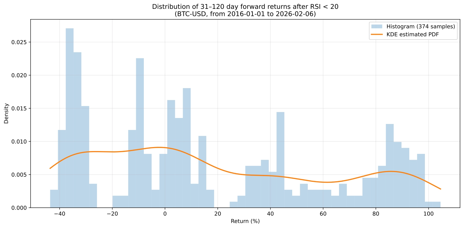
Conclusion for RSI(14) < 20
For RSI below 20, only 18 days were found even across more than a decade, which highlight deep oversold conditions are quite rare! However, it raises the concern how robust is the distributional estimation with such a small sample size. It's also important to note from these 18 days there were 13 in 2018 and these were consecutive days, and 2 of them were in 2023 also consecutive, which means we could acquire only 4 independent events for the analysis, since we don't have data about yesterday's drop.
What can we see from the distribution?
The estimated PDF looks quite flat. It has 3 peaks, one around -35%, one around 0% and one around 85%. This means after an oversold event the outcome of future price movement is quite uncertain. The positive skewness of 0.43 suggests that there is a mild tendency for larger positive returns compared to negative ones, even though the effect is limited by the small sample size. The negative excess kurtosis of -1.12 indicates a platykurtic distribution, meaning the data is flatter than a normal distribution and extreme returns are less frequent than usual. Overall, the distribution signals high uncertainty with only a slight bias toward positive outcomes.
- ➣ Min: -43.59% vs. Max: 104.53% (heavy right tail)
- ➣ Average return: 17.47%
- ➣ Median return: 6.26%
- ➣ Standard deviation: 44.33%
- ➣ Skewness: 0.43 (positive skew)
- ➣ Excess kurtosis: -1.12 (platykurtic distribution)
Conclusion for RSI(14) < 30
For RSI below 30, far more samples were found 134 days, however considering the number of examined days it's still just the ~3.7% of it. But, this is much more reasonable number of events of investigating the distribution, and we can be more confident about the results, even if overlaps are still appears. Besides, the more available sample, data points are more evenly distributed across the examined period, because in this case oversold samples were found in each year.
What can we see from the distribution?
This distribution takes a typical right-skewed bell shape. It almost peaks around 0% return, but it has a long right tail and we can identify extreme returns like +500%. The strong positive skewness of 3.56 highlights that extreme positive returns are much more likely than extreme negative ones, giving the distribution a heavy right tail. The very high excess kurtosis of 15.69 shows a leptokurtic distribution, meaning most returns cluster around the mean but extreme events occur far more frequently than in a normal distribution. This reflects the market's tendency for occasional, very large bullish moves following oversold conditions.
- ➣ Min: -43.59% vs. Max: 517.99% (heavy right tail)
- ➣ Average return: 24.92%
- ➣ Median return: 6.87%
- ➣ Standard deviation: 71.36%
- ➣ Skewness: 3.56 (positive skew)
- ➣ Excess kurtosis: 15.69 (leptokurtic distribution)